Debugging Your Renderer (4/n): End-to-end tests (or, “why did that image change?”)
Here we are, three posts into the meat of this series, and we’re still on the topic of determining if the renderer is buggy in the first place—the actual craft of debugging has not yet seen much discussion. We’re getting there—I promise—but I’m going to finish discussing ways of detecting bugs before getting into fixing them.
Beyond unit tests, I’ve also found that having a good set of end-to-end rendering tests is of enormous benefit. In this context, the idea of an end-to-end test is simple: you render an image of a scene and then check the image to make sure it is correct.
There’s plenty of nuance in that sentence: which scene? (And not just one, right?) How do you check whether the output is correct? Needless to say, it’s “many scenes,” and as we’ll see, verifying correctness from an image can be as much art as science. We’ll dig into all of those questions today.
Building a Library of Test Scenes
I’ve been collecting scenes to use for testing pbrt for at least a decade; there are upward of 600 of them in the test suite today. Most of them don’t make pretty pictures and some output very low resolution images. Some are as small as \(10 \times 10\) pixels—nothing much to look at at all. They can be split into a few categories:
- Simple scenes with analytic solutions.
- Scenes that target a single renderer feature.
- Complex(ish) scenes.
- Reproduction cases for user-reported bugs.
Each type is valuable. Take the scenes with analytic solutions: one such scene is a diffuse sphere with radius 1, a reflectance of 0.5, and a point light with intensity \(\pi\) at its center. Put a camera inside that thing and render it with your path tracer: if your pixels don’t all have a value very close to 1 (given sufficient samples), you’ve got a bug. Stop right there, fix it, and be happy you had such an easy way to detect something was off.
You can take that scene and easily make variations of it. Replace that single point light with four point lights with intensities that sum to \(\pi\)—that should be all ones as well. Or Take out the point light and make the interior of the sphere emissive with spatially- and directionally-uniform radiance of 0.5, leaving the diffuse reflectance at 0.5. Once again, you should get pixels that are all 1. That emissive sphere you can make bigger or smaller; it should be all ones if you make a variant with a different radius.
Once you start thinking in terms of scenes where you can work out the correct answer, there’s lots more you can do. You could light a diffuse quad with an infinite light source and then again with an emissive sphere surrounding it. You could test your bidirectional algorithms by putting a glass where with an index of refraction of 1 around the quad; in principle, that should have no effect.
And then you can also make variants of those variants that exercise all of the different sample generation algorithms and light transport algorithms; each of those is just a small change to the scene description file, so getting up to 600 doesn’t need to go one at a time.
The analytic scenes rarely fail once you’ve gotten them working the first time, but when they do, the debugging problem is a relatively easy one—much nicer than “images of the Moana Island scene are too dark when the bidirectional path tracer is used.” For example, for the scene with a single point light, every ray should return the same value—at each intersection point, the reflected radiance due to direct lighting should be 0.5 and then the indirect radiance (also 0.5) should be scaled by 0.5. (Expand out that series and you get your expected value of 1.)
Of course, those scenes may all render correctly and you may well still find that the Moana Island scene is still too dark with your bidirectional path tracer, but you’ve at least carved off the easy-to-fix cases in a way that makes them easy to debug.
For most of the renderer’s capabilities, it’s not too hard to come up with a simple scene that targets that feature without exercising too many other parts of the renderer. Those are also useful to have in end-to-end tests. As an example, pbrt’s test suite includes a scene comprised of a single quad with a high-frequency texture viewed at an oblique angle. The BSDF is diffuse, it’s lit by a directional light, there’s no complex visibility or multiple light scattering. This is it:
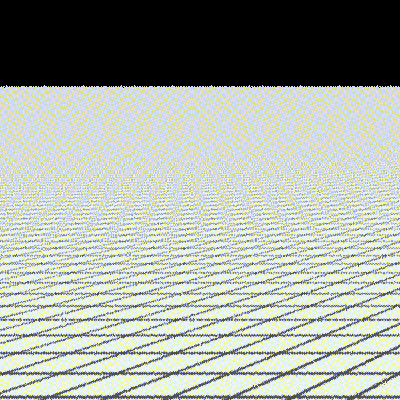
That scene is effectively a test of pbrt’s ray differentials and texture filtering code. If one makes a change to the renderer and then that scene goes bad, you can make a good guess about where the bug lies from the limited subset of the rendering code that runs in generating it. In such a case, if scenes without textures still render correctly then you have a stronger hint, though if those are also broken, then you have a hint that texture filtering isn’t your problem. (Or, that you have multiple problems.)
Sometimes things only go wrong in the presence of complexity; a number of scenes culled from the pbrt-v4-scenes distribution and added to the end-to-end tests take care of that. When those scenes fail, it’s usually the case that simpler ones do as well. If not, it’s often worth trying to simplify the more complex scene as much as possible while still hitting the bug; that, too, is a source of more test scenes for the future. (More on that topic in a future post as well.)
Finally, there are the scenes from user bug reports. I add all of those to the test suite; not only are they all cases that testing previously wasn’t rigorous enough to catch, but there’s no reason to risk the embarrassment (on this end) and annoyance (on the bug reporter’s end) of that same bug reappearing in the future due to a change to the renderer inadvertently reintroducing it.
There is a time versus coverage trade-off in assembling this collection of scenes: the more scenes you have with the more pixels to render and the more samples per pixel, the more you’re exercising the renderer. Yet, the more of all of that you have, the longer it takes to run the tests. If running them takes too long, you won’t run them as often as you should. I’ve ended up tuning them to be about an hour of single-core CPU time (though they run on multiple cores, so it’s just a few minutes of wall-clock time). As you add scenes and the total time to run all of them increases, you can judiciously reduce the resolution of some of the tests or dial down the sampling rate used when rendering them.
Does Everything Render to Completion?
So you have a few tens or hundreds of test scenes and, let’s hope, a script to render all of them and save the images. What now? Run that script and see what happens.
Most of the corners of the renderer’s code ends up being fairly well exercised if you have hundreds of varied scenes designed to exercise it.1 That’s good news for your assertions, as far as giving them plenty of variety to assert about. It’s also encouragement to add more assertions; sometimes adding a new assertion and running through all of the existing test scenes will unearth a new failure. You might even add expensive assertions for a single run-through of the test scenes to see if they find anything, planning to debug if so and to remove them or demote them to debug-only assertions when you’re done.
Finding a failing assertion in that way really is a good thing, even though you’ve found more work for yourself. You’ve got yourself a debugging task ahead of you but it’s not completely open ended, and it’s on your own terms without the panic of a user reporting a serious bug where you have no idea what the cause may be. It’s also likely with a simpler scene than a user would have been rendering if they encountered the bug later.
Assertions aside, the renderer may crash for some or even all of the scenes. Same deal with that: a crash is not fun, but better to find it yourself while running the tests and fix it before your users are bothered by it.
A good collection of test scenes is also good fodder for tools like valgrind, helgrind, and assorted sanitizers. There’s a much better chance of those sorts of tools finding something if you give them a variety of rendering computations to examine. Chasing down any errors those report is also something you must do before proceeding when you find them: there’s no way to know how much havoc lies in their wake, so you might as well fix them once you’re aware of them, lest you spend hours chasing down some other bug that turned out to be due to one of those.
Are the Images Correct?
If all of the scenes render to completion, now you have a few hundred images sitting on disk. How do you know if each one is correct?
For pbrt’s test scenes, I maintain a set of “golden” images that provide a reference.2 The test script then checks the output from the current version of the renderer with the golden images. How tricky could that be? The first hard problem is generating golden images in the first place. The second is determining if a rendered image is correct. We’ll consider both topics in turn.
Creating an initial set of golden images is a bootstrapping problem. For the scenes with analytic solutions you can manually verify correctness via their pixel values, but for the rest it’s not so easy. I have partially been able to sidestep that issue by assuming that the last released version of pbrt is bug free and using its output as a starting point. While pbrt is surely not bug free, after it has been out for a few years enough people have spent enough time with the code that it’s reasonable to assume it’s in pretty good shape.
For a different renderer, one might try using the output of pbrt or another renderer as an initial reference, though that’s tricky business, with differences in BSDF models, texture filtering, and details like rendering in RGB versus using spectra. One can at least make sure that one’s renderer is in the right ballpark that way, if another renderer is both trusted and well-understood and if it’s not too hard to render scenes in both it and your own renderer.
Another option is to gain confidence in candidate golden images via experiments. We’ll come back to this topic in more detail once we get to debugging techniques, but to understand the idea, let’s consider that texture filtering test from before. Say that you’ve implemented ray differentials and a texture filtering algorithm and can render images that aren’t obviously wrong. Lacking a verified solution, how can you become more confident that they are correct?
You might render the scene with no texture filtering but with many pixel samples to get an antialiased image that way. That’s something to compare to. You know that your implementation won’t match that perfectly, but if it’s too far off you might be suspicious of your differentials’ correctness. Another useful technique is to explore the parameter space: render it once with your implementation, then again with your texture filter widths half as wide as you think they should be, then again with them twice as wide. You should see aliasing with the narrow filters and blurring with the wide ones. If so, you have some more confidence in your implementation, and if not, you have something to dig into further.
Here are some images that show the results of applying that approach for the texture filtering test above; the images are as we would expect. (The images are presented using jeri; click on them and hit ‘f’ to go full screen if necessary to see the differences.)
At minimum one may decree that the output of the renderer at some point in time gives the golden images. Going forward, any deviation in them should be explained, either from fixing a bug or from a well-understood improvement to the renderer.
When the Images Should Not Change at All
Given golden images, a change to the renderer, and a run of the end-to-end tests, we have a set of new images that may or may not the match the golden images. How one feels about that depends on the sort of change one has made. Here are a few representative cases where not a single pixel of a single image should be different:
-
A pooled memory allocator was introduced to optimize small memory allocations.
-
An optimized routine for parsing text floating-point values in the scene description was adopted.
-
The function that loads image texture maps has been parallelized to reduce start-up time.
For all of those cases, there’s no reasonable explanation for why anything should change in the final output, yet sometimes you make a change like that and find differences. If it’s major differences, then presumably you’ve broken something fundamental; the debugging problem in those cases is often not too bad due to the wide impact. Choose the one of the simplest scenes that went astray and take it from there.
For minor differences, it’s also critical to understand what happened. It can hard to be disciplined about that: if it’s just one pixel in one scene out of hundreds of scenes with perhaps billions of pixels changes after you replaced the float parser, it’s easy to tell yourself that a single float was parsed differently and hey, quite possibly you just fixed a bug you didn’t know you had. Yet something more serious may be lurking; it may just be that your tests only hit a buggy case once but other scenes would hit it often. If you don’t understand the root cause, you’re building the rest of the system on sand.
For the case of the float parser, it’d be crucial to track down which float (or floats) went astray and why—keep both parsers around, call both for each float parsed, and assert that both give the same result. When they disagree, figure out which one was correct. Your assertion may never fire, which would be “interesting” as well; it may be that the pixel change was not due to a difference in parsing floats but was due to some other bug that was tickled by your changes. Those sorts of bugs aren’t fun to chase down but are equally important to understand when you encounter them.
Implicit in these imperative statements about no pixels changing has been the assumption that the renderer is deterministic—that rendering the same scene gives exactly the same output image. For now we will take that as given. Making the renderer so is tricky but worthwhile; that will be the sole topic of the next post in this series.
When the Images May Change
Whenever changes are made to code involving ray tracing, other geometric computations, or light transport algorithms, it’s almost inevitable that images will change. This brings us to the tricky question of “are those changes ok, or suggestive that there is a bug?”
To motivate this case, let’s consider a (real) example: making what is believed to be an improvement to the algorithm that makes sure that rays leaving bilinear patches do not incorrectly reinstersect the patch. Assuming that we had a reasonable algorithm for this previously, we would expect very small changes in the images for every scene that has bilinear patches in it, but would not expect any big image changes. (Though we might hope to have a scene that shows a case where the current algorithm is insufficient, in which case we would hope for significant and visually evident improvement with it.)
My testing script uses pbrt’s imgtool program to compare the output images to the golden images. It prints nothing when they match exactly, so if you’ve just changed the float parser, you might run the end-to-end tests, wait for them to finish, and move along happily if nothing is reported. When there is a discrepancy, imgtool’s output is like this:

That output is carefully crafted. The three lines in turn:
- The news: the images are different.
- The pathnames of the two images, relative to the current directory. These are there alone and together on a line so that it’s easy to triple click that line to select it, then type the name of an image viewer in the shell, paste the selection, hit return, and then view the two images.
- Numerical details about the images and how they differ.
Those details include the average value of all of the pixels in each image, their percentage difference, and their mean squared difference. Often those numbers alone are enough to indicate what’s going on. If we saw something like the above for all of the test scenes that had bilinear patches in them (minuscule differences in average pixel values and MSE), we could be fairly confident that all was well. It would still be worth a quick glance at a few of the images, but there would be no need to view all of them to feel good about the change.
With that workflow in mind, imgtool offers some color in its output to make it easier to see higher levels of error. Here’s what it said about another scene after I made that change:

That red text says “this seems a little high”, and indeed it is so—here are the corresponding images:
Something funny is happening at the boundary of the liquid at the top of the cup; it is evident that one of two images must be wrong, though it isn’t obvious which one is. Time to start debugging.
Using Statistics to Your Advantage
For the bilinear patch intersection example, the image statistics are useful for giving a good first indicator of “all is well”, “something may be fishy here”, or “things are Not Good.” That is plenty useful, but when one is making changes to Monte Carlo sampling code, those numbers have even greater value. Consider improving a BRDF importance sampling routine to better match the BRDF. In that case, we hope for significant image changes for the better thanks to lower error. How do we distinguish between an improvement in error and an incorrect result?
Just looking at the images may not be enough. Consider these three images of the San Miguel scene where the first is the baseline reference and the others correspond to two different changes to the renderer, one correct and one buggy. It’s not evident from just looking at the images which one is wrong.
However, imgtool has something interesting to report: the average pixel value of “Change A” is 0.17% higher than the reference image, but the average pixel value of “Change B” is 4.03% higher. In the context of unbiased Monte Carlo, a 4% change is most definitely a sign of something going wrong.
One way to think about why this is so is that if you’re using unbiased Monte Carlo algorithms, rendering images of thousands of pixels, each with tens of samples, then you have hundreds of thousands or even millions of sample values that feed into that average. If you have changed your importance sampling routines (and your estimators don’t have ridiculously high variance), then those average image values should be well locked in if both “before” and “after” are bug-free.
That idea also explains why that San Miguel test has a fairly low sampling rate—just 16 samples per pixel. You often don’t need to render the whole image to convergence to tell if the Monte Carlo bits have gone wrong; the statistics over all of the pixels often tell the tale.
But how do you know how much of a change is acceptable? Is that 0.17% something to worry about? In practice, it depends; the answer depends on how many samples you’re taking and how much variance there is in your estimators. For pbrt’s tests, I’ve learned to have a sense of what’s expected, but that’s admittedly imprecise. A much better way would be to follow the ideas presented in Kartic Subr and Jim Arvo’s paper on applying proper statistical tests to these tasks. They show not only the right way to decide if two images have the same mean, accounting for the number of samples taken in setting a threshold, but also showing how to robustly determine the answer to questions like “does image a have lower variance than image b?”
For all of these evaluations of images, it’s crucial that images are stored in floating point, not clamped, and without any tone mapping or gamma correction. When you’re making images for people to look at, you’re more than welcome to use 8-bit PNGs and run your pixels through the ACES curve for a “filmic” look. For the purposes of end-to-end tests, maintaining good old linear values with their full dynamic range is the only thing that allows you to reason about what’s going on with them statistically.
Finally, even if the numbers look good, it’s still important to view the images, or at least all of those ones with the greatest reported differences. A shortcoming of those image-wide statistics is that they don’t indicate whether the error has some unsightly structure to it that is sneaking under the radar. One way to better automate that test would be to also use a perceptual error metric like ꟻlip, though that requires high-quality reference images, which pbrt’s end-to-end tests currently avoid in the interests of running more quickly.
Conclusion
This has turned into a longer post than I intended and there’s still plenty more to say, especially about the tricky problem of having two rendered images and trying to figure out what their differences signify. We will most certainly come back to that in following posts since it is frequently integral to the renderer debugging process.
The best thing about having a good set of tests—both unit and end-to-end—is being able to iterate on code with confidence. You can refactor swaths of the system, you can cleanup things that are a little grungy, and if the tests are clear, you can feel confident about committing those changes. Sometimes you can try out speculative ideas—things where you’re not sure if the idea is right—and quickly gather some empirical data about whether the idea works or not. If those indicators are promising and you pursue your idea you should still find better ways to validate it, but I’ve found that a quick yes/no can be a helpful guide.
Next time we’ll go into the details of making a renderer deterministic, which is one of the foundations of everything discussed today. That post will certainly be less to digest than this one was.
notes
-
The Right Thing to do would be to use a tool that measures code coverage, see which parts of the renderer never or rarely run given your test scenes, and to introduce new scenes intentionally to exercise that code. Admittedly, I have not yet found that discipline for pbrt. ↩
-
Note that the golden images must be generated from scratch for each operating system and compiler used, as differences in details like precision in the system math library usually leads to minor image differences across different systems. ↩