Swallowing the Elephant (Part 8): Meet The GPU
It’s been over three months since my last post about rendering Disney’s Moana Island scene with pbrt-v4. Back then, I promised a further update that would discuss performance when rendering the scene on the GPU, but here we are with months gone by and no further news. Today, finally, I’ll start to rectify that.
Most of the delay was due to lack of motivation: for once, performance was surprisingly good out of the box. Where we left off last time, pbrt-v4’s CPU rendering path was down to 96.8 seconds of wall-clock time between the start of parsing the scene description and the start of actual rendering work. With the GPU path selected and with no further attention to performance tuning, rendering started after 83.3 seconds—1.16x faster.
Of course, faster is to be expected, as roughly half of the pre-rendering time on the CPU is spent building BVHs. pbrt’s BVH construction code is written for clarity rather than performance, is only sort-of parallelized, and runs entirely on the CPU. When rendering on the GPU, all of the BVH construction is handled by highly-optimized code in OptiX, most of it running on the GPU. If using that had been slower than pbrt’s CPU path, then there surely would have been “interesting” things to discover. However, faster was the expectation, and faster was what we got.
Further sapping motivation for blogging, not only was system startup fast, but rendering the scene itself on the GPU pretty much just worked the first time. Here’s the beach view, rendered using an NVIDIA RTX A6000 GPU. I’m going to save the topic of GPU rendering performance for a later post, but, well… It’s most definitely fast.
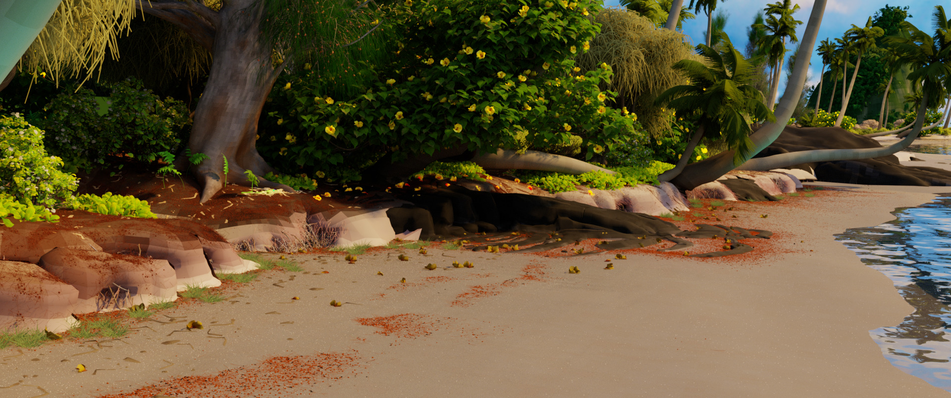 Moana Island beach view rendered with pbrt-v4 on an NVIDIA RTX A6000 GPU with 1024 samples per pixel.
Good performance is always nice, but this series of blog posts has mostly been about chasing down and fixing performance problems due to poor scaling in the face of complexity; everything running well doesn’t leave much to write about. With what I saw at first, I assumed that I would end up with a short post without much technical content that instead declared victory and showed a few pretty pictures. Happily (in a way), once I started actually looking at the data, there were all sorts of good surprises.
The Value of Logging For Finding Stinky Things
I’m all for a good debugger and a good profiler, but it’s surprising
how far one can go with basic instrumentation and logging. For example,
if you give pbrt --log-level verbose in its command-line arguments, it
prints all sorts of chatty information as it does its work, announcing that
it’s starting up the thread pool, telling you what it has found as far as
GPUs in the system, and giving updates about what it’s currently working
on.
Here are a few lines of what it prints early on when rendering the Moana island scene:
[ tid 000 @     0.103s parser.cpp:745 ] Started parsing materials.pbrt
[ tid 000 @     0.103s parser.cpp:620 ] Finished parsing materials.pbrt
[ tid 000 @     0.103s parser.cpp:590 ] Started parsing isMountainA/isMountainA.pbrt
[ tid 000 @     0.103s parser.cpp:590 ] Started parsing isMountainB/isMountainB.pbrt
[ tid 000 @     0.103s parser.cpp:590 ] Started parsing isGardeniaA/isGardeniaA.pbrt
[ tid 000 @     0.103s parser.cpp:745 ] Started parsing isMountainA/objects.pbrt
In each line we get the id of the thread that issued the log message (here,
always the main thread), the elapsed time since pbrt started running, the
location in the source where the logging call was made, and then whatever
it has to tell us. Here we can immediately see that the entirety of
materials.pbrt was parsed nearly instantaneously. We can
also see that multiple additional files are being parsed in parallel, each
getting started without pbrt waiting for the one before it to finish. This all
is to be expected, so no surprises so far.
As I was gearing up to start writing this post, I noticed the following when doing
a run with --log-level verbose:
[ tid 000 @    43.820s wavefront/integrator.cpp:140 ] Starting to create lights
[ tid 000 @    53.465s wavefront/integrator.cpp:229 ] Done creating lights
That’s ten seconds to create the light sources in the scene. Those ten seconds were especially evident when seen live—there’s “Starting to create lights”, then no logging whatsoever for ten long seconds before pbrt comes back, bright eyed and proud that it’s gotten all the lights taken care of. That long pause was enough for me to realize something was off; I knew that it had been no more than 5 or so seconds to create the lights for this scene before, so there was surely something amiss.
While a profiler could have cleared up what was happening in those ten seconds, a simple sampling-based approach was enough: I re-ran pbrt (still using an optimized build) with the debugger, waited for that long ten second pause, then stopped execution and printed out the current stack trace before letting it resume.1 A few quick iterations of that was all it took to discover that much of that time was spent in two functions that checked whether an image had any pixels with floating-point infinity or not-a-number values.
I had added those checks after spending way too much time debugging an unexpected infinity that turned out to be from an environment map light source that had an infinite-valued pixel. Now, the Moana island scene includes an environment map that is 8k pixels square, otherwise known as 64 million pixels. Oh, and those pixels are stored as 8-bit values, so there’s no risk of funny floating-point values in any of them. Perhaps looping over all of them, lovingly converting them from 8-bit sRGB to float, and then seeing if they were perhaps infinite was not the best use of cycles.
It took two one-line fixes to early out in that case, and light creation time went back to the 5 seconds or so that it used to be. The total time to first pixel went down to 77.9 seconds—19 seconds faster than when rendering with the CPU.
Basic Profiling in the Renderer
Fixing that self-inflicted wound gave me some momentum; it was a small taste of the satisfaction of making something slow run faster and that was enough to give me motivation to dig in further. However, the task is trickier than it was before since pbrt is now doing work on both the CPU and the GPU. It’s important to understand what each is up to; for example, maybe it’s fine if the CPU is mostly idle at some point if the GPU is working full-tilt. However, if both are lounging around not doing much, then perhaps we should see where the slacking lies.
Sticking with my log-based methodology, I added a --log-utilization
command-line
option
to pbrt. It causes an extra thread to be launched that measures current
system activity every 100ms and reports it to pbrt’s verbose log. Thus,
when it’s running, you get updates ten times as a second about what’s going
on interspersed with pbrt’s regular logging output, which makes it easy to
connect to what pbrt is doing. Here’s what it reports at the start of
light creation:
[ tid 000 @    43.213s pbrt/wavefront/integrator.cpp:140 ] Starting to create lights
[ tid 000 @    43.267s pbrt/util/log.cpp:175 ] CPU: Memory used 32101 MB. Core activity: 0.0155 user 0.0000 nice 0.0000 system 0.9845 idle
[ tid 000 @    43.267s pbrt/util/log.cpp:193 ] GPU: Memory used 1156 MB. SM activity: 0 memory activity: 0
[ tid 000 @    43.367s pbrt/util/log.cpp:175 ] CPU: Memory used 32101 MB. Core activity: 0.0140 user 0.0000 nice 0.0016 system 0.9845 idle
[ tid 000 @    43.368s pbrt/util/log.cpp:193 ] GPU: Memory used 1156 MB. SM activity: 0 memory activity: 0
[ tid 000 @    43.468s pbrt/util/log.cpp:175 ] CPU: Memory used 32101 MB. Core activity: 0.0155 user 0.0000 nice 0.0000 system 0.9845 idle
[ tid 000 @    43.469s pbrt/util/log.cpp:193 ] GPU: Memory used 1156 MB. SM activity: 0 memory activity: 0
Both CPU and GPU activity are reported where a value of 1 represents full utilization. The system I’m using has a 32 core/64 thread CPU, so all 64 of those threads would need to be active and doing work to achieve a 1. Here, we can see that we’ve got one thread keeping busy (1/64=0.0156), with everything else sitting idle. That’s not impressive, but it’s not unexpected: there’s little parallelism in that part of the system.
Just as with the regular text logging, I often find it productive to eyeball that output. Though it’s not as fancy as a graphical profiler, there’s nearly zero overhead to using it; sometimes, low friction is more important than comprehensive data. Reading such logs is actually how I did all of the work described in this and the two following posts, though it’s also easy enough to make graphs using that output as well.
First Performance Graphs and Setting a Baseline
As a baseline, here is where things stood with the light creation fix in there, shown using separate graphs for the CPU and the GPU.2 These graphs start after the scene description has been parsed and materials, textures, and lights have been created. For these investigations we’ll focus on the geometric work that happens after all that finishes, starting 47 seconds in. Up until then both the CPU and GPU path run the same code, which has probably received enough attention for now.
Here, x axis is time in seconds and the y axis is processor utilization. The start of rendering is indicated by a vertical dashed line.


Four phases of work that are shown in these graphs:
- Process non-instanced geometry: all of the non-instanced geometry (e.g., the mountains and the ocean surface) is converted to objects like pbrt’s
TriangleMesh, including reading geometry that stored in PLY files from disk. Once this geometry is in memory, pbrt has OptiX build BVHs for it. (Triangles and non-triangles go into separate BVHs.) - Build instance BVHs: For each geometric object that is instanced (e.g., each type of shrub and flower), the geometry is read from disk and an individual BVH is built.
- Process instance uses: For each use of a geometric instance, a structure is initialized that bundles up the handle to the instance’s BVH and the transformation matrix that places it in the scene.
- Build top-level BVH: The final scene-wide BVH is built including both the non-instanced geometry and all of the instance uses.
Going back to the graphs, the only thing to be happy about is the final stage of building the final top-level BVH: there’s not much left for the CPU to do at that point and the GPU is nicely occupied during that phase. For worse and for better, there’s plenty of unused computing capacity left sitting idle in the rest of the graph.
A First Small Victory
The nearly 6 seconds spent on Process instance uses was one of the first
things that caught my eye, even though it’s not where most of the time is
spent. If you look at the corresponding
loop,
there’s not much to it; there’s a hash table lookup using the name of the instance
(e.g. “xgCabbage_archivecoral_cabbage0003_geo”). That leads to the handle to
its BVH and then there’s just a bit of data movement, initializing an
OptixInstance structure with the transformation matrix and a few other
things so that the instance use is part of the final scene BVH.
Since that loop is not doing much that is computationally intensive, it didn’t seem worth parallelizing when I first wrote it. However, when you have over 39 million instances, a little bit of data movement for each one adds up. It’s easy enough to parallelize that loop: (1) (2), and doing so brings Process instance uses down from 5.9 seconds to 1.1 seconds of wall-clock time, which brings us to 72.2 seconds for time to first pixel. These graphs show the improvement:


(As in earlier posts, the scale of the x axis is the same as the baseline graph in order to make it easier to compare successive graphs with each other.)
CPU utilization during that phase is still a little spiky, but that phase now achieves the best CPU utilization of all of them. With its total time down to one second, it’s hard to worry too much more about it.
Looking Ahead
It was a slow start, but we’ve gone from lack of motivation to two easy fixes that shaved roughly ten seconds off of startup time. Furthermore, those have brought us to being “just” twelve seconds away from a sub-one-minute time to first pixel. That would be exciting, and there’s still got plenty of idle processor time in the graphs and plenty of code still unexamined under the lens of Moana. To that end, we’ll dig into the instance BVH phase next time around.
notes
-
I’m not sure where I first learned about this trick. I’m almost certain that I read a blog post extolling the idea somewhere years ago but am unable to find it again now. ↩
-
The GPU’s performance monitoring API reports its results averaged over an unspecified but up-to-one-second amount of previous time whereas the CPU numbers are calculated strictly based on activity in the last 100ms. This leads to some lag in the GPU results that manifests itself in activity sometimes being charged to the wrong stage; an example is “Process instance uses”, which doesn’t actually use the GPU at all. (I also believe that the spike in GPU activity at the start of “Build instance BVHs” should be charged to “Process non-instanced geometry.”) However, rather than futzing with the data, I have reported it as measured. ↩