Visualizing Warping Strategies for Sampling Environment Map Lights
(I know, there’s supposedly another post on sampling triangular light sources coming. Soon, maybe!)
Recent papers on importance sampling have increasingly often started to include visualizations of how various sampling techniques warp the canonical \([0,1)^n\) domain of samples that are used to drive them. Eric Heitz’s recent paper on sampling the GGX distribution is one example; see his Figure 7.
Understanding the way that sample warping algorithms distort the uniform samples that they start out with is important: in general, we’d like to provide them with well-distributed sample points (e.g. from a low-discrepancy point set) and we’d like the warping algorithm to not mess up that distribution—ideally, it should smoothly distort from \([0,1)^n\) to the target domain without discontinuities and without stretching much more in one direction than the other. (This is why Pete Shirley’s “square to disk” mapping generally gives lower integration error than the standard polar mapping of samples to the disk. More details.)
Inspired by recent papers, I decided it would be interesting to make some visualizations to better understand the differences between algorithms used for sampling environment map light sources. Environment maps are generally used to define a light “at infinity”—in other words, an emissive object that is infinitely far away, such that the radiance \(L\) arriving at a point is purely a function of direction \(\omega\). In general, a good importance sampling approach for these lights is to warp samples from \([0,1)^2\) to directions \(\omega\) with probability density proportional to the luminance of each pixel scaled by the solid angle it covers.
Two Warping Algorithms
There are two widely-used approaches for sampling directions according to an environment map light source’s distribution:
- A two-step algorithm based on first sampling a marginal PDF to select a scanline of the environment map and then sampling a conditional PDF along the chosen scanline to select a pixel.
- A hierarchical warping algorithm that uses a MIP-map over the environment map to progressively warp 2D samples until they match the desired distribution.
The first approach is described in Physically Based Rendering; see the linked section for details. Most of the implementation is in pbrt’s Distribution2D class.
The second approach is described in the paper Wavelet Importance Sampling: Efficiently Evaluating Products of Complex Functions, by Clarberg et al. (While that paper is mostly about a technique for sampling according to the product of BSDF and the environment map, their sample warping algorithm can be applied to the environment map alone.) They apply a series of linear warps of the form \(f(x) = a(x-b)\) to the \([0,1)^2\) domain, alternating between the two dimensions. They take advantage of the fact that because MIP map texels store averages of the texels in a region of the image, looking at relative averages shows how to progressively warp the \([0,1)^2\) domain to match the image.
This figure from their paper gives a flavor of the idea:
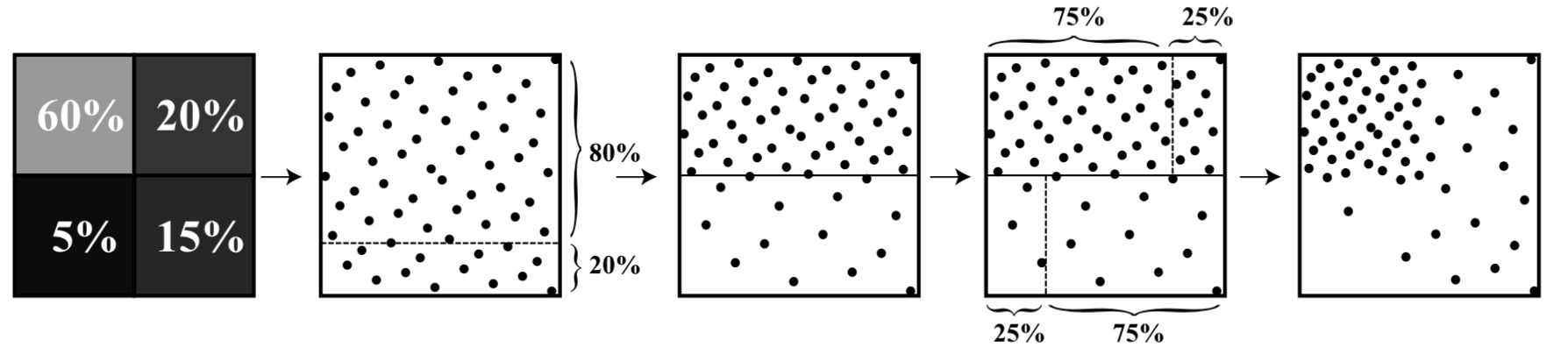 The first step of the hierarchical sample warping algorithm: the four pixel
values from the first MIP level below the root give the relative fraction
of samples that should be allocated to the corresponding quarters of the
image. In turn, the sampling domain is warped accordingly,
here first in y and then in x. Further linear warpings are applied at each
successive MIP level.
The first step of the hierarchical sample warping algorithm: the four pixel
values from the first MIP level below the root give the relative fraction
of samples that should be allocated to the corresponding quarters of the
image. In turn, the sampling domain is warped accordingly,
here first in y and then in x. Further linear warpings are applied at each
successive MIP level.
Here’s my implementation of the hierarchical warping algorithm (.h, .cpp.) It comes from the next version of pbrt, so it doesn’t compile as is, but I don’t think it’d be too hard to get it working, especially as part of the current version of pbrt.
Visual Comparison of Distortion
In order to better understand how the two warps work in practice, I created some visualizations of how they distort strata from the \([0,1)^2\) sample domain. I split the domain into \(16 \times 16\) strata and assigned a different color to each one, which has us starting out with this:
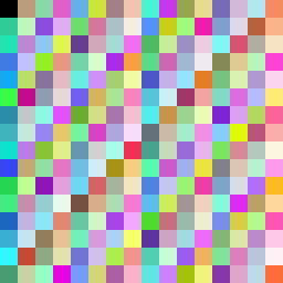
Then for both mappings, I computed the inverse mapping: for each pixel in the environment map, I determined which sample value in \([0,1)^2\) mapped to that pixel, and in turn colored the environment map pixel according to the strata colors above. The resulting images give a sense of how the original strata are distorted by the warping.
I chose three environment maps from HDRI Haven for evaluation: Snowy Park 01, Surgery, and Qwantani. They range from having relatively uniform illumination (Snowy park) to localized extremely bright illumination (Qwantani). Surgery is somewhere in the middle.
Here are the results, via jeri. They’re best viewed on a laptop or desktop computer. Click on the tabs to switch between the environment maps and the visualizations. After selecting the image below, I encourage you to hit ‘f’ to go full screen in order to be able to see the details well. Hit ‘?’ to see a list of all of the keyboard shortcuts.
The thing to look for in these visualizations is “how are the strata distorted?” (and in turn, “how do I feel about that?”)
The results are… interesting.
Snowy park is a fairly straightforward case. Visually, I think that the hierarchical warp does best here, mostly maintaining pretty much rectangular strata. I see at least one case where part of a stratum has been sheared off and is disconnected from the rest of it, but otherwise it looks pretty good. The 2D warp goes a bit wavy; what we’re seeing is adjacent scanlines with significantly different sampling distributions so that the second sampling step warps the points very differently from scanline to scanline. Nevertheless, all of the original strata remain connected, which is a good thing.
The results are along similar lines for Surgery though there we can see the differences between how the two warping functions pull samples to the bright lights. With the hierarchical warp, we see fairly distorted strata all around the lights, where the distortion happens in both dimensions. With the two dimensional warp, the scanlines with bright lights have that same wavy distortion we saw with Snowy park, just much more so.
Finally, there’s Qwantani. The sun is about 150,000 times brighter than the blue sky around it and therefore much of the sampling domain is pulled toward the sun’s direction. With the hierarchical warp, we can see that quite a few strata have been broken into pieces and many of the remaining ones are stretched much more in one dimension than the other. The 2D warp has plenty of its own distortion, though for better or for worse, it’s localized in the scanlines that include the sun and its reflection.
Conclusion? I don’t know—warping’s hard. Rendering tests with those three environment maps indicate that both warping functions give similar error, so there’s no clear winner between them on that front, either. “Use whichever approach is most efficient on your target architecture” is all I’ve got to offer for a conclusion for today.