Adventures in Sampling Points on Triangles (Part 1)
Illumination from area lights is one of those wonderful things that just works with path tracing; a nice big light source gives realistic soft lighting that matches most real-world lighting much better than a couple of point lights, for example. Part of using Monte Carlo integration to estimate direct lighting from an area light involves choosing a point on the light source’s surface, tracing a shadow ray to it, and adding a contribution from the light if the shadow ray is unoccluded.
Regular practice is to generate a random (or, better, quasi-random) 2-dimensional point in [0,1)2 and apply a transformation that warps the canonical [0,1)2 domain to the surface of the light source. (A variety of these warpings are cataloged in Section 13.6 of Physically Based Rendering.)
These warpings are normally designed to minimize distortion: as much as possible, we’d like nearby sample points to remain nearby after the transformation to the light’s surface. This is particularly important if carefully-constructed sample points like low-discrepancy samples are being used; a good transformation can maintain the error-reducing properties in their distribution, which in turn reduces error.
Some distortion can’t be avoided in cases where we’re warping between significantly different domains. For example, if we’re mapping from the square [0,1)2 domain to a triangle, some pinching or a folding is unavoidable. I’ve always not worried much about those distortions: I have assumed it wasn’t something that made much of a difference in practice, and didn’t think there was much to do about it once you’d chosen a decent mapping.
As it turns out, I was wrong about all of that, and that’s what we’ll dig into today.
Previous State of the Art
Consider sampling a point on a triangular light source: most commonly,
people use a mapping that takes a 2-dimensional sample u and
gives the barycentric coordinates of a point inside the triangle, sampled
with uniform probability—in other words, all points on the triangle are
chosen with equal probability if the sample u is uniformly
distributed. Here’s its implementation:
std::array<float, 3> UniformSampleTriangle(const Point2f &u) {
    float su0 = std::sqrt(u[0]);
    float b0 = 1 - su0;
    float b1 = u[1] * su0;
    return { b0, b1, 1.f - b0 - b1 };
}
Let’s see how using that mapping works out in practice. Here’s a plot of 64 pmj02bn sample points, which were described in Christensen et al.’s EGSR paper last year. I think they’re the best two-dimensional sample points out there at the moment. They’re carefully optimized to satisfy a number of useful properties, including the power-of-2 elementary intervals and not clumping together too much.
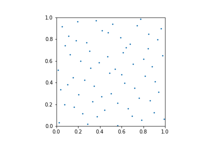
64 pmj02bn sample points.
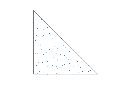
It’s a good looking point set. Now let’s map those points to a triangle, using the mapping defined above. Here’s what we get:
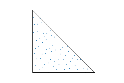
64 pmj02bn sample points mapped to a triangle.
It’s fine, but if you want to pick nits, you can find some things to be unhappy about: here and there you can find clusters of a few points that are fairly close together, and there are also some pretty big areas that don’t have any points at all in them.
Basu and Owen’s Mapping
In 2014, Kinjal Basu and Art Owen published a paper, Low discrepancy constructions in the triangle. The fact that I just read it a few weeks ago is a pretty good indication of what a dumpster fire my reading pile is.
Their approach is based on mapping a 1-dimensional sample in [0,1) onto the surface of the triangle—already we have something new and thought-provoking going on, their not using a 2-dimensional sample. They use the digits of the base-4 digital representation of that number to select a point inside the triangle in a way that’s reminiscent of choosing a point along a space-filling curve and in turn get pretty nicely-distributed points.
To make the idea concrete, say that we have a (base ten) sample value of 0.125. Converted to base 4, we have 0.02. (The first digit to the right of the radix point is contributes its value times 1/4, the second contributes its value times 1/16, and so forth. Thus, we have 0/4 + 2/16 = 1/8, our original sample value.)
Given the sample value in base 4, their mapping considers its digits in turn, from most to least significant. The first digit is used to choose one of four sub-triangles, illustrated on the left side of this figure (from their paper). Next, the second digit is used to choose a sub-triangle within that sub-triangle (shown on the right), and so forth. For our 0.125 sample, we end up with that “02” sub-triangle on the right.
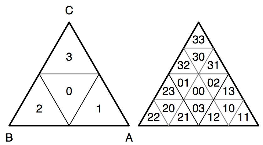
How digits in the base-4 sample value are successively
used to select sub-triangles in the original triangle. Here, the
sub-triangles for the first digit (left) and first and second digits
(right) are shown.
Here are 64 samples generated using this approach. Note that they are fairly evidently more evenly distributed than the warped pmj02bn points, though there’s also some visible structure to them.
64 samples in a triangle generated using Basu and Owen's algorithm.
Sample Points and Randomization
The 1-dimensional sample points used for their mapping must be chosen carefully. Basu and Owen use the van der Corput points, which in base 4 are 0.0, 0.2, 0.1, 0.3, 0.02, etc. Given a power-of-four number of such sample points, we can see that each applicable sub-triangle will be selected exactly once.
How important is it to use those points? Here’s what happens if you use their mapping using 64 stratified one-dimensional samples:
Sample points
generated using regular stratified samples with Basu and Owen's mapping.
Their distribution is much worse than if van der Corput points are
used.
You get a much worse distribution of sample points, even though thanks to stratification, each of the 64 applicable sub-triangles still has exactly one sample in it. Thus, we can see that both the points and the mapping are key to their method.
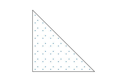
In turn, you might ask yourself how much of the benefit from their approach comes from the sample points being regularly distributed and whether the traditional approach could benefit from more of that. For a sense of that, here’s what happens if a regular grid of unjittered sample points is put through the traditional mapping. The distortion introduced by the mapping is fairly easily seen.
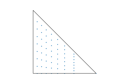
64 2-dimensional samples in a regular grid, using the traditional
mapping. The mapping's distortion is evident.
One would still like some variation in the points sampled on the triangle from pixel to pixel—we’d see structured error in images if we didn’t somehow randomize the samples across pixels. One approach that doesn’t destroy the mapped points’ distribution is to apply a Cranley-Patterson rotation to the one-dimensional sample points before mapping them to the triangle. The idea is to add an offset in [0,1), different at each pixel but the same for all samples in a pixel, and to then use the fractional part of the result to sample a point in the triangle:
    u += delta;  // delta between 0 and 1
    if (u > 1) u -= 1;
A good way to compute those offsets is with blue noise textures which ensure that nearby pixels have significantly different offsets, which in turn leads to error being manifested with high-frequency noise, which is visually pleasing.
Implementation
The implementation of Basu and Owen’s technique is pretty straightforward. Given a sample value in [0,1), we first multiply by 232 and convert to an integer, effectively giving us a 0.32 fixed-point base-2 representation of the sample.
Here’s the start of the implementation:
std::array<Float, 3> LowDiscrepancySampleTriangle(Float u) {
    uint32_t uf = u * (1ull << 32);           // Convert to fixed point
We maintain the barycentric coordinates of the three corners of the current
sub-triangle using variables A, B, and C, taking advantage of the
fact that we only need to track two barycentric coordinates for each one,
since we can always get the third by subtracting the other two from 1. We
can extract the base-4 digits just by taking pairs of those binary digits.
    Point2f A(1, 0), B(0, 1), C(0, 0);        // Barycentrics
    for (int i = 0; i < 16; ++i) {            // For each base-4 digit
        int d = (uf >> (2 * (15 - i))) & 0x3; // Get the digit
Given the digit, there are a series of rules (given in the paper) that give the updated barycentrics.
        Point2f An, Bn, Cn;
        switch (d) {
        case 0:
            An = (B + C) / 2;
            Bn = (A + C) / 2;
            Cn = (A + B) / 2;
            break;
        case 1:
            An = A;
            Bn = (A + B) / 2;
            Cn = (A + C) / 2;
            break;
        case 2:
            An = (B + A) / 2;
            Bn = B;
            Cn = (B + C) / 2;
            break;
        case 3:
            An = (C + A) / 2;
            Bn = (C + B) / 2;
            Cn = C;
            break;
        }
        A = An;
        B = Bn;
        C = Cn;
    }
And finally, when we’re out of digits, we just take the sample at the center of the small sub-triangle that we’re in:
    Point2f r = (A + B + C) / 3;
    return { r.x, r.y, 1 - r.x - r.y };
}
Results
The sample points on the triangle look nice enough, but how do things work out with actual rendering? Here’s a simple scene, rendered with 16 samples per pixel, using pmj02bn points, and multiple importance sampling. The two images below show the difference between the traditional mapping and the new one.
(Click on the tabs to switch images, or use the number keys after selecting the image. Hit ‘f’ to go fullscreen. You can also pan and zoom using the mouse.)
The reduction in noise is fairly obvious. The second image actually has 2.17x less variance than the first one. (And recall, that means that the first image would need 2.17x more rays to achieve the same error.) Success!
Now, this is admittedly a scene that is favorable to the method: if the light source was small, for example, the benefit would be less. Still, it’s a pretty nice improvement for not too much more work.
Next time, we’ll consider applying this approach to sampling spherical triangles, which gets interesting in its own ways.