Re-reading An Introduction to Ray Tracing
I recently re-read An Introduction to Ray Tracing on the occasion of its recent release in a free online edition. And to be clear, I read my physical copy, a first printing from 1989, since I’m OG like that.
I don’t remember what I paid for my copy, but it was a college-student purchase. Whatever it cost, it could have been a lot of pizza and beer instead. No regrets, even then.
It’s hard to over-state the importance of this book to my own computer graphics education. I can’t guess how many times I read it; it’s the sort of book I read and re-read, absorbing a little more each time.
It’s remarkably cohesive for a book that is a collection of chapters by different authors. Books like that sometimes turn out to be mishmashes where at each chapter break you can tell that someone new is taking over, not having paid too much attention to what came before and not worried too much about what’s coming after. An Introduction to Ray Tracing doesn’t suffer any of that.
I don’t know if it’s that Andrew Glassner, the book’s editor, wielded a strong pen, or if the authors all knew this stuff so well that they naturally self-organized to present the right ideas to get the reader going down the path. Maybe it was some of both.
It’s worth a read today—all of it. The basics are presented more clearly than one might expect for an idea that was, for graphics, just eight years old at the time. I’ve found that reading the work from the early days can be the most illuminating, as it hasn’t become all fouled up with jargon and gratuitous complexity. There’s also a pioneering aspect, the “we’re still working out the details so please bear with us,” that ends up making it more approachable. You can play along at home, knowing more now about how it all turned out.
A lot of the content is still familiar—for example, the basics of ray–object intersection remain the same today. It’s fun to see how much has changed, though: for example, of 88 pages over two chapters on ray–object intersection algorithms by Eric Haines and Pat Hanrahan, there are only nine pages on ray–polygon intersection, and the special case of ray–triangle gets less than a page in total. All the rest of those pages are about things like intersecting the good old quadrics, CSG, surfaces of revolution, implicit surfaces, and other things that don’t seem so important today.
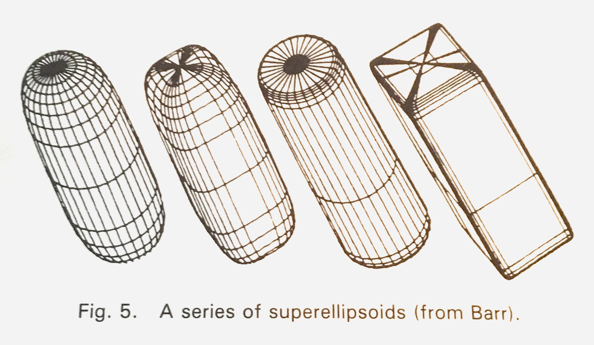
A few objects that are of somewhat less interest to be intersected than they once were.
The chapter on acceleration structures by Jim Arvo and David Kirk is also chock-full with choice. It gives the reader a sense of how active an area of research that was and how little of it was settled then. Arvo and Kirk present all sorts of spatial and primitive subdivisions, augmented with variations that also account for ray direction in the hierarchies, some approaches based on making use of ray coherence, and discussion of the possibilities from tracing beams and cones instead of just rays.
In spite of the uncertainties of what was the best data structure, how to build it was already clear: not only is the surface area heuristic there, but there’s a discussion of its assumptions and limitations that is still insightful today.
Rob Cook’s chapter on stochastic sampling and distribution ray tracing is probably my favorite, for two reasons. The first is that he gives a remarkably clear discussion of jittering, why it has the filtering characteristics it has, and how it turns aliasing into noise, that via the simple example of considering the effect of jittered sampling of sine waves of various frequencies.
The second reason relates to rendering depth of field. Starting on page 178, Cook starts to explain how to transform polygons in screen space given a sample point on a thin lens in order to account for depth of field. By the time you get to page 186, he’s explained how to bound polygons in screen space given a particular thin lens aperture size.
You might be wondering, what does that have to do with ray tracing? To be honest, I have no idea. Then and now, to render depth of field in a ray tracer you just adjust your camera ray origin based on lens position and take it from there. Screen space has nothing to do it—that only matters if you’re rasterizing. However, as far as I know, those pages are the only place that information is written down and explained clearly. In addition to valuing the content, I like the subversion of sneaking some rasterization heresy into a ray tracing book.
The book wraps up with Writing a Ray Tracer, by Paul Heckbert. It includes an extended outline of ray tracer features. Structured using a clear taxonomy, it captures all sorts of features one might want to implement. It starts slow, with things like “special case shadow rays so that shading calculations aren’t performed for them” and then warms up to “add support for motion blur,” “use spectra rather than RGB,” all the way up to “add support for distributed computing across multiple machines.” It’s comprehensive in terms of 1989 ray tracer features, and was a source of inspiration when I wrote my own early ray tracers.
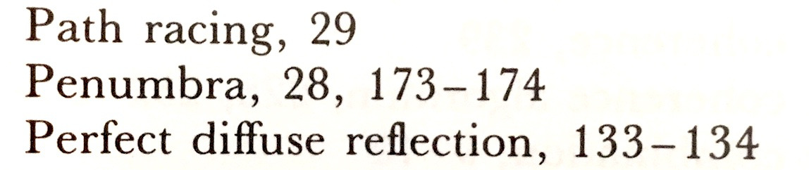
Today, the most striking thing to me is that both the rendering equation and path tracing are only mentioned in passing, and then only a few times. There’s never any suggestion that you’d actually use that stuff to make images. At most, you might do distribution ray tracing with a little jitter at the lens, a little jitter in time, and a little jitter for reflections—that’s about as much of sampling the full path space as could be imagined to be practical. Path tracing only appears once in the index, and there with the indignity of an unfortunate typo:
The section on parallel and vector architectures for ray tracing at the end of Arvo and Kirk’s chapter helps illuminate why path tracing saw so little attention.
A representative architecture that they describe is a parallel ray tracing system that used Intel 8087 floating-point units. For grounding, those ran at 4 MHz and offered 50,000 FLOPS. For the reader who is unfamiliar with “FLOPS” without a “G” or a “T” at the start, they are just plain old floating-point operations, counted one at a time but still measured per second. A good GPU today offers about 50,000,000 times more of them. Put another way, a computation you can do today in 1/1000 of a second you could do on an 8087 in about 14 hours.
With that kind of performance available from CPUs, specialized hardware was of interest. In that same section of the book, there’s also discussion of a hardware architecture for ray tracing introduced by Ullner in his 1983 Ph. D. dissertation:
The performance […] was quite impressive (for 1983), being able to compute a new ray–polygon intersection every 1/3 microsecond once the pipe was full. […] It would thus be able to exhaustively ray trace an anti-aliased 512x512 image containing 1000 polygons in approximately 10 minutes.
Perhaps the best thing of all from a re-reading is the understanding of how far we’ve come.